Advanced Example

In this second example, we will take a look into a couple more advanced features and ways to customize Cockpit.

Note

Just like before, you also need the utility file which provides us with the training data, a convolutional network and a logpath. You can copy all example files from our repository.

"""A slightly advanced example of using Cockpit with PyTorch for Fashion-MNIST."""

import torch
from _utils_examples import cnn, fmnist_data, get_logpath
from backpack import extend, extensions

from cockpit import Cockpit, CockpitPlotter, quantities
from cockpit.utils import schedules

# Build Fashion-MNIST classifier
fmnist_data = fmnist_data()
model = extend(cnn())  # Use a basic convolutional network
loss_fn = extend(torch.nn.CrossEntropyLoss(reduction="mean"))
individual_loss_fn = extend(torch.nn.CrossEntropyLoss(reduction="none"))

# Create SGD Optimizer
opt = torch.optim.SGD(model.parameters(), lr=5e-1)

# Create Cockpit and a plotter
# Customize the tracked quantities and their tracking schedule
quantities = [
    quantities.GradNorm(schedules.linear(interval=1)),
    quantities.Distance(schedules.linear(interval=1)),
    quantities.UpdateSize(schedules.linear(interval=1)),
    quantities.HessMaxEV(schedules.linear(interval=3)),
    quantities.GradHist1d(schedules.linear(interval=10), bins=10),
]
cockpit = Cockpit(model.parameters(), quantities=quantities)
plotter = CockpitPlotter()

# Main training loop
max_steps, global_step = 50, 0
for inputs, labels in iter(fmnist_data):
    opt.zero_grad()

    # forward pass
    outputs = model(inputs)
    loss = loss_fn(outputs, labels)
    losses = individual_loss_fn(outputs, labels)

    # backward pass
    with cockpit(
        global_step,
        extensions.DiagHessian(),  # Other BackPACK quantities can be computed as well
        info={
            "batch_size": inputs.shape[0],
            "individual_losses": losses,
            "loss": loss,
            "optimizer": opt,
        },
    ):
        loss.backward(create_graph=cockpit.create_graph(global_step))

    # optimizer step
    opt.step()
    global_step += 1

    print(f"Step: {global_step:5d} | Loss: {loss.item():.4f}")

    if global_step % 10 == 0:
        plotter.plot(
            cockpit,
            savedir=get_logpath(),
            show_plot=False,
            save_plot=True,
            savename_append=str(global_step),
        )

    if global_step >= max_steps:
        break

# Write Cockpit to json file.
cockpit.write(get_logpath())

# Plot results from file
plotter.plot(
    get_logpath(),
    savedir=get_logpath(),
    show_plot=False,
    save_plot=True,
    savename_append="_final",
)

To run this example script, run

python 02_advanced_fmnist.py

This time no Cockpit-plot will show. Instead, the plots will be directly saved to files. Everything that the Cockpit tracked during training will also be stored and both this logfile as well as the plots can be inspected and analyzed after training is finished.

$ python 02_advanced_fmnist.py

Step:     1 | Loss: 2.2965
Step:     2 | Loss: 2.3185
Step:     3 | Loss: 2.2932
Step:     4 | Loss: 2.2893
Step:     5 | Loss: 2.2865
Step:     6 | Loss: 2.2780
Step:     7 | Loss: 2.2485
Step:     8 | Loss: 2.2600
Step:     9 | Loss: 2.1823
Step:    10 | Loss: 2.0557
[cockpit|plot] Saving figure in ~/logfiles/cockpit_output__primary10.png
Step:    11 | Loss: 2.0539
Step:    12 | Loss: 2.4792
[...]

We will now go over the main changes compared to the basic example. The relevant lines including the most important changes are highilghted above.

Network Architecture

model = extend(cnn())  # Use a basic convolutional network

In contrast to the basic example, we use a convolutional model architecture instead of a dense network. For Cockpit this does not change anything! Just like before, the network needs to be extended, which works in exactly the same way as before.

Customizing the Quantities

# Create Cockpit and a plotter
# Customize the tracked quantities and their tracking schedule
quantities = [
    quantities.GradNorm(schedules.linear(interval=1)),
    quantities.Distance(schedules.linear(interval=1)),
    quantities.UpdateSize(schedules.linear(interval=1)),
    quantities.HessMaxEV(schedules.linear(interval=3)),
    quantities.GradHist1d(schedules.linear(interval=10), bins=10),
]
cockpit = Cockpit(model.parameters(), quantities=quantities)

Cockpit allows you to fully customize what and how often you want to track it.

Instead of using a pre-defined configuration, here, we customize our set of quantities. We use five quantities, the GradNorm, the Distance and UpdateSize, the HessMaxEV and the GradHist1d. For each quantity we use a different rate of tracking, e.g., we track the distance and update size in every step, but the largest eigenvalue of the Hessian only every third step. We further customize the gradient histogram by specifying that we only want to use 10 different bins.

Additional BackPACK Extensions

        extensions.DiagHessian(),  # Other BackPACK quantities can be computed as well

Cockpit uses BackPACK for most of the background computations to extract more information from a single backward pass. If you want to use additional BackPACK extensions you can just pass them using the with cockpit() context.

Plotting Options

    if global_step % 10 == 0:
        plotter.plot(
            cockpit,
            savedir=get_logpath(),
            show_plot=False,
            save_plot=True,
            savename_append=str(global_step),
        )

    if global_step >= max_steps:
        break

# Write Cockpit to json file.
cockpit.write(get_logpath())

# Plot results from file
plotter.plot(
    get_logpath(),
    savedir=get_logpath(),
    show_plot=False,
    save_plot=True,
    savename_append="_final",
)

In this example, we now create a Cockpit view every tenth iteration. Instead of showing it in real-time, however, we directly save to disk. At the end of the training process, we write all Cockpit information to a log file. We can then also plot from this file, which we do in the last step.

Writing and then plotting from a log file allows Cockpit to not only be used as a real-time diagnostic tool, but also to examine experiments later or compare multiple runs by contrasting their Cockpit views.

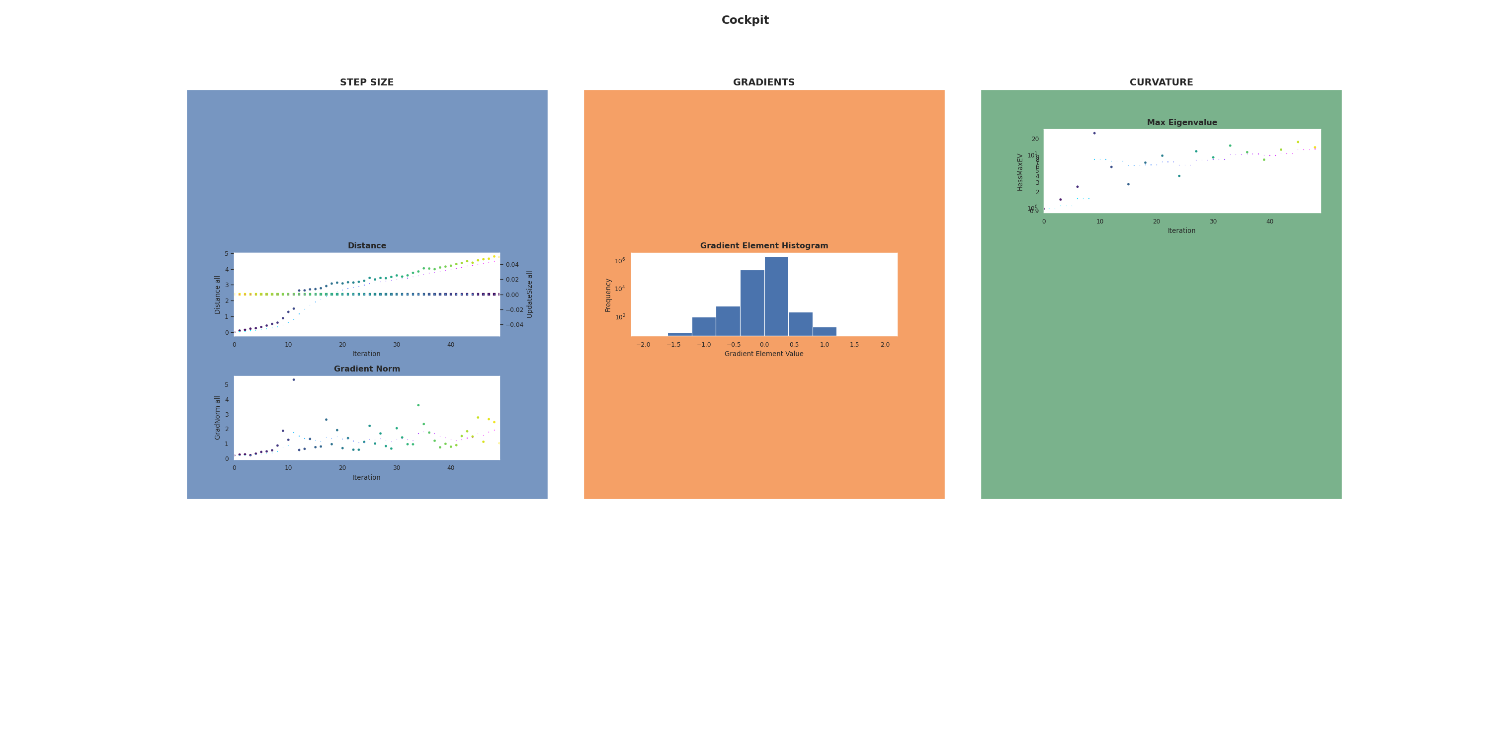
The final Cockpit plot gets also saved and will look similar to the below image. You can see that the CockpitPlotter only shows the instruments where the corresponding quantities have been tracked.