Basic Example

This snippet below shows an example of using Cockpit with a standard PyTorch training loop. Lines that are highlighted in yellow highlight Cockpit-specific code, but don’t worry, most of these changes are simple plug-and-play solutions.

You can try out this basic example yourself. Simply install Cockpit via

pip install cockpit-for-pytorch

and then copy the example files from the repository or from the code block below.

Note

Don’t forget the utility file which provides the data for this example.

"""A basic example of using Cockpit with PyTorch for Fashion-MNIST."""

import torch
from _utils_examples import fmnist_data
from backpack import extend

from cockpit import Cockpit, CockpitPlotter
from cockpit.utils.configuration import configuration

# Build Fashion-MNIST classifier
fmnist_data = fmnist_data()
model = extend(torch.nn.Sequential(torch.nn.Flatten(), torch.nn.Linear(784, 10)))
loss_fn = extend(torch.nn.CrossEntropyLoss(reduction="mean"))
individual_loss_fn = torch.nn.CrossEntropyLoss(reduction="none")

# Create SGD Optimizer
opt = torch.optim.SGD(model.parameters(), lr=1e-2)

# Create Cockpit and a plotter
cockpit = Cockpit(model.parameters(), quantities=configuration("full"))
plotter = CockpitPlotter()

# Main training loop
max_steps, global_step = 5, 0
for inputs, labels in iter(fmnist_data):
    opt.zero_grad()

    # forward pass
    outputs = model(inputs)
    loss = loss_fn(outputs, labels)
    losses = individual_loss_fn(outputs, labels)

    # backward pass
    with cockpit(
        global_step,
        info={
            "batch_size": inputs.shape[0],
            "individual_losses": losses,
            "loss": loss,
            "optimizer": opt,
        },
    ):
        loss.backward(create_graph=cockpit.create_graph(global_step))

    # optimizer step
    opt.step()
    global_step += 1

    print(f"Step: {global_step:5d} | Loss: {loss.item():.4f}")

    plotter.plot(cockpit)

    if global_step >= max_steps:
        break

plotter.plot(cockpit, block=True)

Try running this example script via

python 01_basic_fmnist.py

During every iteration of the training process, Cockpit will show you a status screen of the training.

$ python 01_basic_fmnist.py

Step:     1 | Loss: 2.5365
[cockpit|plot] Showing current Cockpit.
Step:     2 | Loss: 2.1643
[cockpit|plot] Showing current Cockpit.
Step:     3 | Loss: 1.9929
[cockpit|plot] Showing current Cockpit.
Step:     4 | Loss: 1.9733
[cockpit|plot] Showing current Cockpit.
Step:     5 | Loss: 1.6479
[cockpit|plot] Showing current Cockpit.
[cockpit|plot] Showing current Cockpit. Blocking. Close plot to continue.

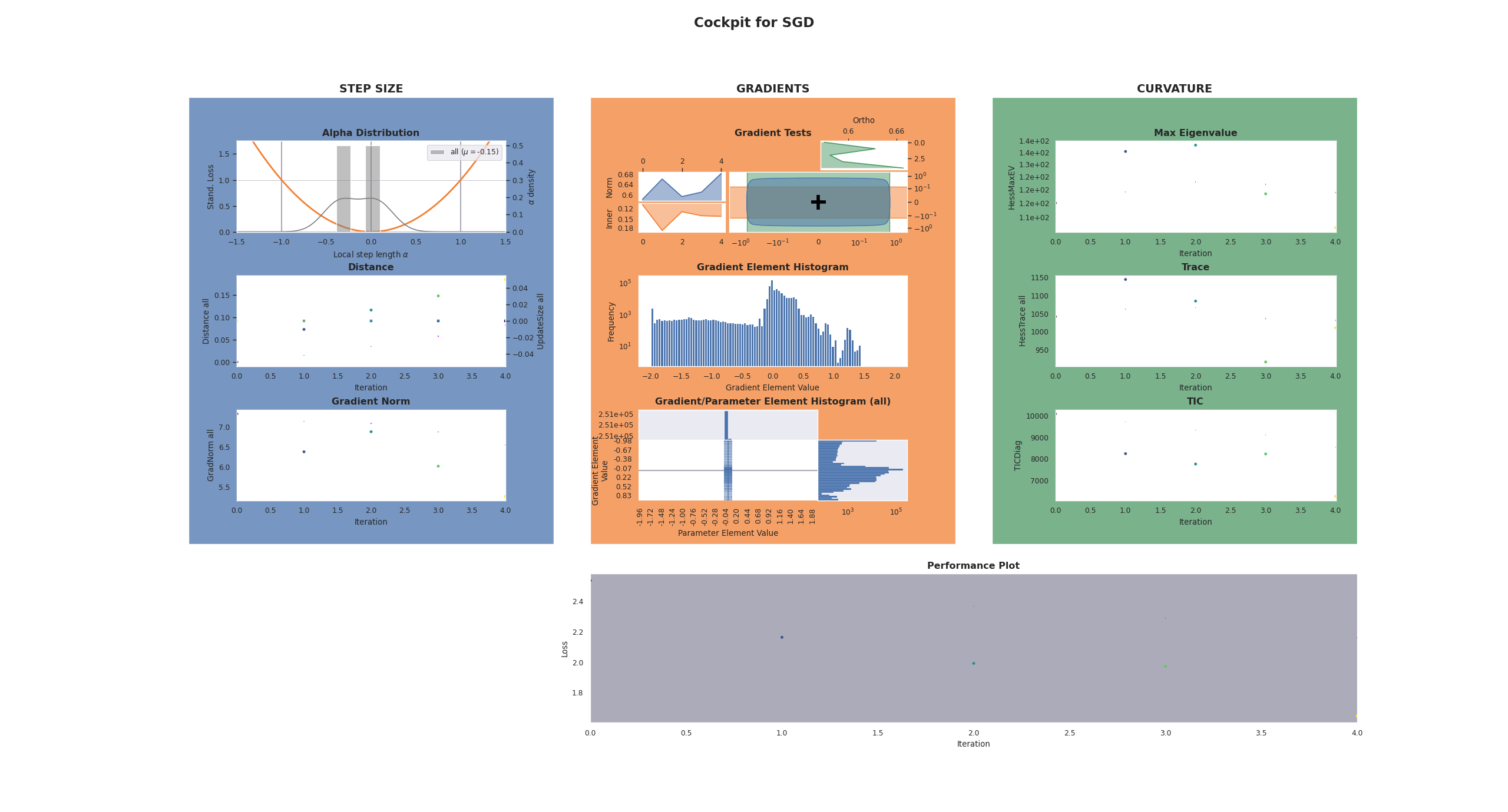
which will look something like this

In the following, we will break-down and explain each step of this exampe, which also explains what is required to include Cockpit to a training loop.

Imports

"""A basic example of using Cockpit with PyTorch for Fashion-MNIST."""

import torch
from _utils_examples import fmnist_data
from backpack import extend

from cockpit import Cockpit, CockpitPlotter
from cockpit.utils.configuration import configuration

Additionally to importing PyTorch, we import BackPACK which will automatically be installed when installing Cockpit. We also import the Cockpit and CockpitPlotter class which will let us track and then visualize insightful quantities.

To simplify the code snippet, in line 4, we import from a utils file which will provide us with the Fashion-MNIST data.

Defining the Problem

# Build Fashion-MNIST classifier
fmnist_data = fmnist_data()
model = extend(torch.nn.Sequential(torch.nn.Flatten(), torch.nn.Linear(784, 10)))
loss_fn = extend(torch.nn.CrossEntropyLoss(reduction="mean"))
individual_loss_fn = torch.nn.CrossEntropyLoss(reduction="none")

Next, we build a simple classifier for our Fashion-MNIST data set.

The only change to a traditional training loop is that we need to extend both the model and the loss function using BackPACK. This is as simple as wrapping the traditional model and loss function in the extend() function provided by BackPACK. It lets BackPACK know that additional quantities (such as individual gradients) should be computed for these parameters.

For the Alpha quantity we also require access to the individual loss values, which can be computed cheaply but is not usually part of a conventional training loop. We can create this function analogously to the regular loss function just setting the reduction=None. There is no need to let BackPACK know about its existence, since these losses will not be differentiated.

Configuring the Cockpit

# Create Cockpit and a plotter
cockpit = Cockpit(model.parameters(), quantities=configuration("full"))
plotter = CockpitPlotter()

Computation of the quantities and storing of the results are managed by the Cockpit class. We have to pass the model parameters, and a list of quantities, which specify what should be tracked and when.

Cockpit offers configurations with different computational complexity: "economy", "business", and "full" (see also configuration()). We will use the provided utility function to track all possible quantities.

Training Loop

    opt.zero_grad()

    # forward pass
    outputs = model(inputs)
    loss = loss_fn(outputs, labels)
    losses = individual_loss_fn(outputs, labels)

    # backward pass
    with cockpit(
        global_step,
        info={
            "batch_size": inputs.shape[0],
            "individual_losses": losses,
            "loss": loss,
            "optimizer": opt,
        },
    ):
        loss.backward(create_graph=cockpit.create_graph(global_step))

Training itself is straightforward. At every iteration, we draw a mini-batch, compute the model predictions and losses, then perform a backward pass and update the parameters.

The main differences with Cockpit is that the backward call is surrounded by a with cockpit(...) context, that manages the extra computations during the backward pass. Additional information required by some quantities is passed through the info argument.

Plotting the Cockpit

    print(f"Step: {global_step:5d} | Loss: {loss.item():.4f}")

    plotter.plot(cockpit)

At any point during the training, here we do it in every single iteration, the computed metrics can be visualized by calling the plotting functionality of the CockpitPlotter via plot().

    if global_step >= max_steps:
        break

plotter.plot(cockpit, block=True)

After the final iteration, we will again show the full Cockpit view. The option block=True allows us to pause our program and inspect the plot for as long as we want. The final Cockpit status screen will look similar to this:

Simply closing the plotting window ends the program and this example.